Can we find a general theory for randomized smoothing? We show that for an appropriate notion of “optimal”, the best smoothing distribution for any norm has level sets given by the Wulff Crystal of that norm.

In the previous post, we discussed how to learn provably robust image classifiers via randomized smoothing and adversarial training, robust against $\ell_2$ adversarial perturbations. There, the choice of Gaussian for the smoothing distribution would only seem most natural. What if the adversary is $\ell_p$ for $p \ne 2$? What kind of distributions should we smooth our classifier with? In this post, we take a stroll through a result of our recent preprint Randomized Smoothing of All Shapes and Sizes that answers this question, which curiously leads us to the concept of Wulff Crystals, a crystal shape studied in physics for more than a century. Empirically, we use this discovery to achieve state-of-the-art in $\ell_1$ provable robustness in CIFAR10 and Imagenet.

Introduction

While neural networks have excelled at image classification tasks, they are vulnerable to adversarial examples; imperceptible perturbations of the input that change the predicted class label (Szegedy et al. 2014), as illustrated by the following image from Madry and Schmidt’s blog post.

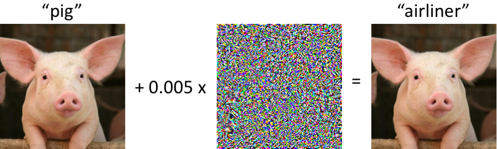
This has most often been formalized in terms of the following desiderata: Let $\mathcal{B}$ be a set of “allowed adversarial perturbations,” such as $\mathcal{B} = \{v \in \mathbb{R}^d: \|v\|_\infty\leq 8/255\}$. Consider a classifier $f$ that maps an input $x$ (e.g. an image) to one of a number of classes (e.g. the label “cat”). Then we say a function $f$ is robust at $x$ to perturbations from $\mathcal B$ if $f(x)$ and $f(x+v)$ share the same labels for all $v \in \mathcal B$.

It is easy to create such inputs by perturbing a data point $x$ by, for example, projected gradient descent (Madry et al. 2018) (see our previous post for a concise overview). This raises important safety concerns as machine learning is increasingly deployed in contexts such as healthcare and autonomy.

The community has developed a plethora of techniques toward mending a model’s vulnerability to adversarial examples: adversarial training, gradient masking, discretizing the input, etc. Yet these “empirical defenses” are usually short-lived and completely broken by newer, more powerful attacks (Athalye et al. 2018).

This motivates the study of certifiably robust defenses, which have emerged to stop this escalating arm race. In such a defense, the classifier not only labels the input, but also yields a certificate that says “not matter how the input is perturbed by a vector in $\mathcal B$, my label will not change.”

We focus on randomized smoothing, a method popularized by Lecuyer et al. 2018, Li et al. 2018, and Cohen et al. 2019 that attains state-of-the-art certifiable robustness guarantees. The core idea is simple: given a classifier $f$ and input $x$, instead of feeding $x$ directly to $f$, we can sample lots of random noise, say from a normal distribution, $(\delta^{(1)},\dots,\delta^{(m)}) \sim N(0, \sigma^2 I)$, and output the most commonly predicted class among the predictions $f(x+\delta^{(1)}),\dots,f(x+\delta^{(m)})$. It turns out that this scheme can guarantee this most common class stays unchanged when the input $x$ is perturbed by vectors of small $\ell_2$ norm. We will more formally discuss this technique below. For more background, we also welcome the reader to see our previous post.

For the most part, prior works on randomized smoothing has focused on smoothing with a Gaussian distribution and defending against $\ell_2$ adversary, neglecting other traditionally important threat models like $\ell_\infty$ or $\ell_1$. Here, we take a step back and ask the following:

What’s the optimal smoothing distribution for a given $\ell_p$ norm?

In answering, we will achieve state-of-the-art empirical results for $\ell_1$ robustness on CIFAR-10 and ImageNet datasets. In the table below we show the certified accuracies comparing our choice of smoothing with the Uniform distribution to the previous state-of-the-art which performed smoothing with the Laplace distribution. Here, each percentage indicates the fraction of the test set for which we both 1) classify correctly and 2) guarantee there is no adversarial example within the corresponding $\ell_1$ radius.

ImageNet	$\ell_1$ Radius	0.5	1.0	1.5	2.0	2.5	3.0	3.5	4.0
	Uniform, Ours (%)	55	49	46	42	37	33	28	25
	Laplace, Teng et al. (2019) (%)	48	40	31	26	22	19	17	14

CIFAR-10	$\ell_1$ Radius	0.5	1.0	1.5	2.0	2.5	3.0	3.5	4.0
	Uniform, Ours (%)	70	59	51	43	33	27	22	18
	Laplace, Teng et al. (2019) (%)	61	39	24	16	11	7	4	3

Background

Let us first introduce some background on randomized smoothing.

Definition. Let $\mathcal Y$ be a finite set of labels (e.g. “cats”, “dogs”, etc). Let $f:\mathbb{R}^d\mapsto \mathcal{Y}$ be a classifier that outputs one of these labels given an input. Given a distribution $q$ on $\mathbb R^d$, we can smooth $f$ with $q$ to produce a new classifier $g$, called the smoothed classifier, which is defined at any point $x \in \mathbb R^d$ as

$g(x) = \underset{c \in \mathcal{Y}}{\arg \max}\ \underset{\delta \sim q}{\mathrm{Pr}} [f(x + \delta)=c].$

A moment of thought should show that $g$ is the same classifier as the one produced by the “majority vote” procedure for randomized smoothing described in the introduction, if we have an infinite number of random noises $\delta^{(1)}, \delta^{(2)}, \ldots \sim q$.

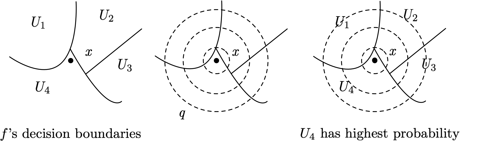
Slightly less intuitively, we can also define $g(x)$ in the following way, in terms of the decision regions of the base classifier $U_c = \{ x' \in \mathbb{R}^d : f(x') = c\}$:

$g(x) = \underset{c \in \mathcal{Y}}{\arg\max}\ q(U_c - x).$

Here $q(U) = \mathrm{Pr}_{\delta\sim q}[\delta \in U]$ and $U_c-x$ denotes the translation of $U_c$ by $-x$. Note $q(U_c - x)$ is the same as the measure of $U_c$ under the recentered distribution of $q$ at $x$, and $g(x)$ is the maximum such measure over all decision regions $U_c, c \in\mathcal Y$.

Now let’s turn our attention to what robustness properties arise in $g(x)$, the smoothed classifier. To do so, we’ll need to consider the worst case over all possible decision regions $U_c$ that may arise, since the base classifier is an arbitrary neural network.

Definition. The growth function $\mathcal G$ with respect to distribution $q$ is defined as,

$\mathcal{G}_q(p, v) = \sup_{U\subseteq \mathbb{R}^d: q(U)=p}q(U-v), \text{for any } p \in[0, 1], v \in \mathbb{R}^d$

Its interpretation is: out of all sets $U$ (i.e. all possible decision regions) with initial measure $p$, what is the most that its measure can increase when we shift the center of $q$ by a vector $v$? Note this is a property of $q$ alone and does not depend on $x$.

For example, consider a 2D Gaussian measure $q = N(0,I)$ with a perturbation $v=[1,1]$. Let $p=\frac{1}{4}$ and consider two possible choices: let $U_1$ be the bottom-left quadrant and $U_2$ be the top-right quadrant. They both have measure $p=\frac 1 4$ under $q$. It’s easy to see that after a shift in the distribution’s center by $v$, $U_2$ will have higher measure than $U_1$.

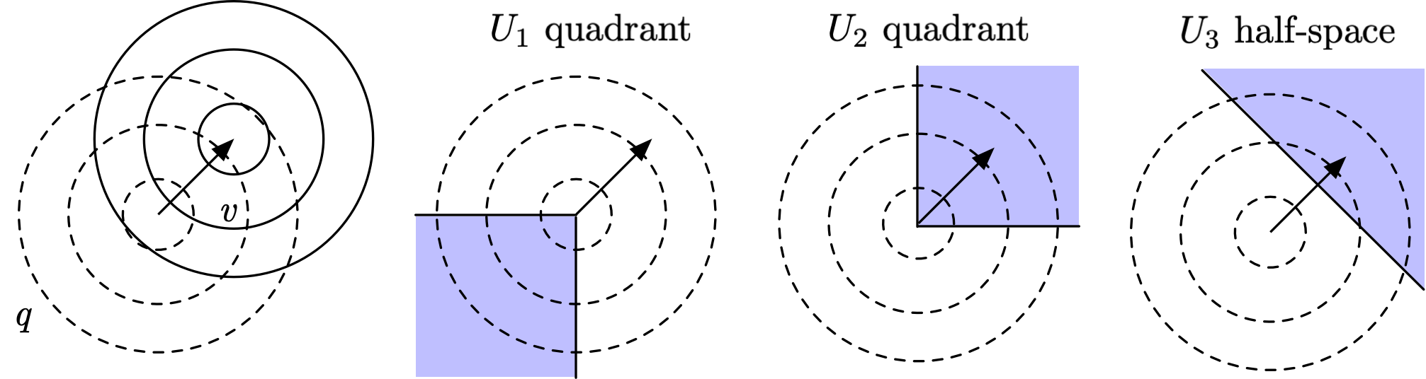
It turns out that here the most extreme choice of $U$ with measure $p=\frac{1}{4}$, in terms of maximizing the growth function, is $U_3$, the half-space formed with a hyper-plane perpendicular to $v$, with boundary positioned such that $q(U_3)=\frac{1}{4}$.

To see this, think of the problem of finding the most extreme $U$ as a problem of “maximizing value under budget constraint.” Each vector $u$ added to $U$ will “cost” $q(u)$, and the total cost is at most $p$, the measure of $U$ under $q$. At the same time, each $u$ will also bring in a “profit” of $q(u-v)$, and the total profit is $q(U-v)$, the measure of $U$ under $q(\cdot -v)$. Thus a greedy cost-benefit analysis would suggest that we sort all $u \in \mathbb R^d$ by $\frac{q(u -v)}{q(u)}$ in descending order, and add to $U$ the top $u$s until we hit our cost budget, i.e. $\int_{U} q(u)du = p$. In the above example of $q$ being Gaussian, the ratio $\frac{q(u -v)}{q(u)}$ changes only along the direction $v$ and stays constant in each hyperplane perpendicular to $v$, so the above reasoning confirms that the half-space $U_3$ above is the maximizing $U$. The growth function in this example would then read $\mathcal G_q(\frac 1 4, v) = q(U_3-v)$, which turns out to have a simple expression that we shall describe below.

If the smoothed classifier $g$ assigns label $c$ to input $x$, then $U_c - x$ has the largest measure under $q$ among all decision regions $\{U_c: c \in \mathcal Y\}$. Thus, $g(x+v) = g(x)$ if $U_c-x$ does not shrink in $q$-measure too much when it is shifted by $-v$, or equivalently if the complement of $U_c-x$ does not grow too much in $q$-measure. This intuition can be captured more formally with the growth function:

Result. Suppose for a base classifier $f$, we have $\rho = \mathrm{Pr}_{\delta \sim q}[f(x+\delta) = c] > \frac{1}{2}$. Then the smoothed classifier $g$ will not change its prediction under perturbation set $\mathcal{B}$ if

$\sup_{v\in\mathcal{B}} \mathcal{G}_q(1-\rho, v)< \frac{1}{2}.$

Back to our 2D Gaussian example, and suppose we have $\rho=1-p=0.75$ and recall that we’re interested in a perturbation $v=[1,1]$. From the above result we know that $g$ will not change its prediction as long as $\mathcal{G}_q\left(1-0.75, [1,1]\right)<\frac{1}{2}$. So we need to calculate $\mathcal{G}_q\left(0.25, [1,1]\right)$, which is the measure of the half-space we identified earlier, under the distribution $q$ shifted by $[1,1]$. Where is the boundary of the half-space? Consider a change of basis so that the x-axis follows the direction of $v$ such as in the center figure below. The boundary occurs at $x=\Phi^{-1}\left(0.75\right)$. What’s the measure of this half-space under $q$ shifted by $[1,1]$? Exactly $1-\Phi(\Phi^{-1}(\frac{3}{4}) - \sqrt{2})$.

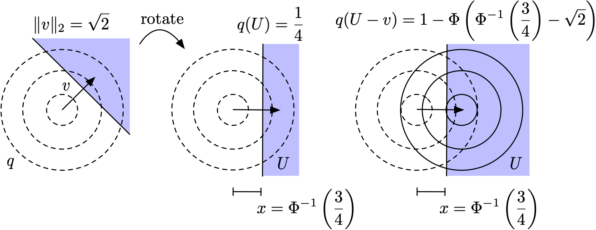
Therefore,

$\mathcal{G}_q\left(0.25, [1, 1]\right)= 1-\Phi\left(\Phi^{-1}\left(0.75\right)-\sqrt 2\right) \approx 0.77 > 0.5,$

so the classifier is not robust to the perturbation if $\rho=0.75$. On the other hand, following similar logic we can calculate the growth function for $\rho=0.99$, which tells us

$\mathcal{G}_q(0.01, [1,1]) = 1 - \Phi(\Phi^{-1}(0.99)-\sqrt 2) \approx 0.41 < 0.5,$

so the classifier is robust to the perturbation if $\rho=0.99$.

More generally Gaussian smoothing yields the bound derived in Cohen et al. 2019,

$\mathcal{G}_q(1-\rho,v) = 1-\Phi\left(\Phi^{-1}(\rho) - \frac{\|v\|_2}{\sigma}\right).$

The Optimal Smoothing Distributions

Here we provide intuition for the question we want to answer:

What is the best distribution to smooth with if we want $\ell_p$ robustness?

First let’s simplify and consider a uniform distribution over a convex set $S\subseteq \mathbb{R}^d$ where $\mathrm{Vol}(S)=1$. By inspection,

$\mathcal{G}_q(p,v)=\min(1, p + \mathrm{Vol}((S + v) \setminus S)).$

In this situation, the $U$ that obtains the $\sup$ for the growth function is any subset of $(S + v )\cap S$ with volume $p$, unioned with the complement of $S$. For example, see the left figure below, in which the area of $U \cap S$ is $p$, satisfying $q(U)=p$ where $q$ is the measure of our uniform distribution.

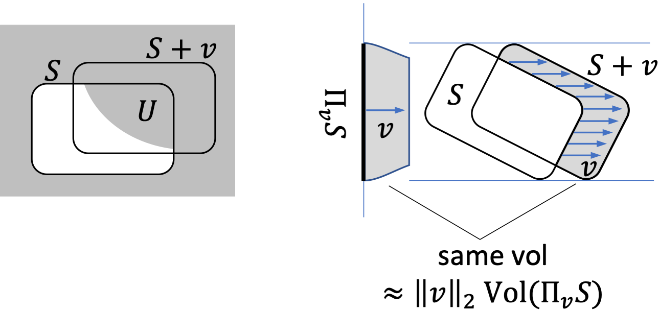
Now consider an infinitesimal translation by $rv$. As $r\rightarrow 0$, the volume of $(S + v) \setminus S$ approaches $r$ times the volume of the projection $\Pi_v S$ of $S$ along $v$, in terms of $(d-1)$-dimensional Lesbegue measure. Here, $\Pi_v S$ is formally defined as $\{u - \frac{u^\top v}{\|v\|^2} v: u \in S\}$. See the right figure above for an example in 2D – the projection $\Pi_v S$ of $S$ along $v$ yields the length between the two blue horizontal lines.

This intuition justifies the following limits:

$\lim_{r\rightarrow 0} \frac{\mathcal{G}_q(p, rv) - p}{r} = \lim_{r\rightarrow 0}\frac{\mathrm{Vol}((S+rv)\setminus S)}{r}= \|v\|_2\mathrm{Vol}(\Pi_v S).$

In the context of randomized smoothing, recall that the smoothed classifier is robust to a perturbation $v$ as long as $\mathcal{G}_q(1-\rho,v)<\frac{1}{2}$. Here in our uniform distribution example, this means that $g$ is robust to small perturbations $rv\in r\mathcal{B}$ as long as

$\begin{aligned} \mathcal{G}_q(1-\rho, rv) & \approx 1-\rho + r\| v\| _2 \mathrm{Vol}(\Pi_v S) < \frac{1}{2}\\ \iff & r < \frac{\frac{1}{2} - (1-\rho)}{\|v\|_2\mathrm{Vol}(\Pi_vS)}. \end{aligned}$

If we consider the worst-case perturbation $rv\in r \mathcal{B}$ for a fixed model, we have a smoothed classifier robust to a perturbation set $\mathcal{B}$ as long as

$\sup_{rv\in r\mathcal{B}}\mathcal{G}_q(1-\rho,rv) \approx 1-\rho + r\sup_{v\in\mathcal{B}}\|v\|_2\mathrm{Vol}(\Pi_v S) <\frac{1}{2}.$

Importantly, the model is more robust as $\sup_{v\in\mathcal{B}}\|v\|_2 \mathrm{Vol}(\Pi_v S)$ decreases. So a natural question to ask is, which set $S$, our smoothing distribution, minimizes this quantity over all convex sets of volume $1$?

It turns out the answer is the Wulff Crystal, a shape from theoretical physics.

Wulff Crystals

Definition. The Wulff Crystal with respect to $\mathcal{B}$ is defined as the unit ball of the norm dual to $\|\cdot\|_\ast$, where $\|x\|_\ast= \mathbb{E}_{y\sim\mathrm{Vertices}(\mathcal{B})} \vert x^\top y \vert$ with $y$ sampled uniformly from vertices of $\mathcal{B}$.

Let’s unpack this a bit. Recall dual norm is defined as,

$\|z\| = \sup \{ z^\top x : \|x\|_\ast \leq 1\}.$

For example, it’s well known that the dual norm of the $\ell_p$ norm is the $\ell_q$ norm where $\frac{1}{p} + \frac{1}{q} = 1$.

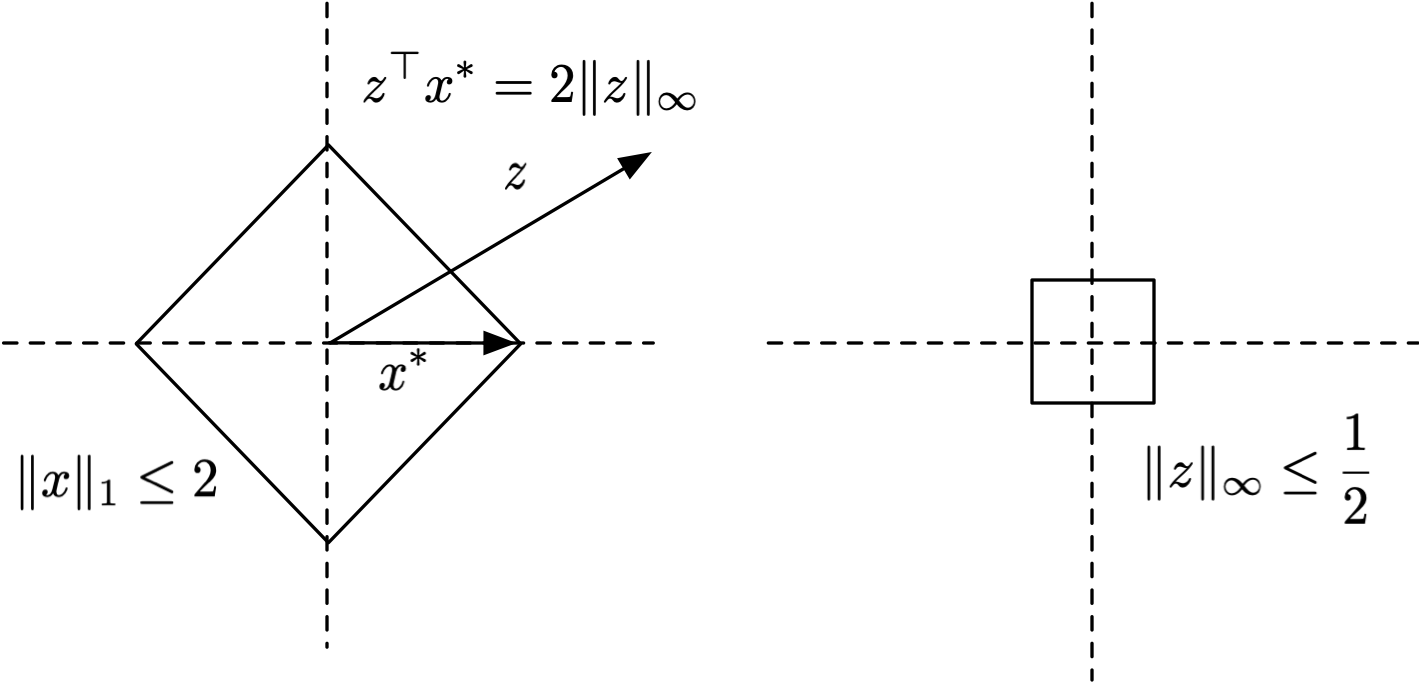
Now suppose we’re interested in the Wulff Crystal for $\mathcal{B}$, where $\mathcal{B}$ is the $\ell_1$ rhombus in two dimensions, which has vertices $\{ (0, 1), (0, -1), (1, 0), (-1, 0)\}$. Thus,

$\begin{aligned} \mathbb{E}_{y\sim \mathrm{Vertices}(\mathcal{B})}|x^\top y| & = \frac{1}{2}|x_1| + \frac{1}{2}|x_2| \end{aligned}$

So the constraint $\|x\|_\ast \leq 1$ corresponds to constraining $\|x\|_1 \leq 2$ i.e. a scaled version of the $\ell_1$ rhombus. What’s the dual of this? For any $z$, $\sup\{z^\top x:\|x\|_1 \leq 2\}=2\|z\|_\infty$, so the Wulff Crystal is the ball $\|z\|_\infty\leq \frac{1}{2}$.

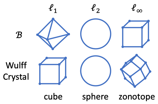
Below we show a few examples of Wulff Crystals for different perturbation sets $\mathcal{B}$.

• For the $\ell_1$ cross-polytope, the Wulff Crystal is a cube.
• For the $\ell_2$ sphere, the Wulff Crystal is a sphere.
• For the $\ell_\infty$ cube, the Wulff Crystal is the zonotope (i.e. Minkowski sum) of vectors $\{\pm 1\}^d$. In two dimensions this is a rhombus and in three dimensions it is a rhombic dodecahedron, but in higher dimensions there is no simpler description of it than as the zonotope of the vectors $\{\pm 1\}^d$.

Result. For any $p \in [0, 1)$, the Wulff Crystal with respect to $\mathcal{B}$ minimizes the quantity

$\sup_{v\in\mathcal{B}}\lim_{r\rightarrow 0} \frac{\mathcal{G}_q(p, rv) - p}{r} = \sup_{v\in\mathcal{B}}\lim_{r\rightarrow 0} \frac{1}{r}\mathrm{Vol}((S + rv) \setminus S)$

among all measurable (not necessarily convex) sets $S$ of the same volume, and when $\mathcal{B}$ is sufficiently symmetric (e.g. $\ell_1,\ell_2,\ell_\infty$ balls).

In other words, setting $S$ to be the Wulff Crystal minimizes the growth function, and therefore makes $g$ more robust. So this covers cases of smoothing with a distribution that’s uniform over a set $S$. What about the more general (i.e. non-uniform) case? It turns out the Wulff Crystal remains optimal, in that it determines the best shape of the distribution’s level sets.

Result. Let $q_0$ be any reasonable distribution with an even density function. Among all reasonable and even density functions $q$ (i.e. $q(x) = q(-x)$) with superlevel sets $\{x: q(x) \geq t\}$ with the same volumes as those of $q_0$, the quantity

$\sup_{v\in\mathcal{B}}\sup_{q(U)=\frac{1}{2}} \lim_{r\rightarrow 0 } \frac{q(U-rv)-\frac{1}{2}}{r}$

is minimized by the distribution $q^\ast$ with superlevel sets proportional to the Wulff Crystal with respect to $\mathcal{B}$. For proof, see our paper.

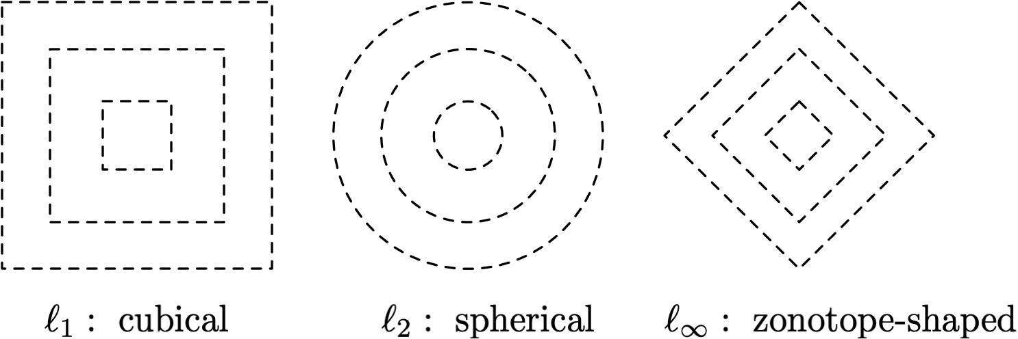
This means that:

• For the $\ell_1$ ball, the distribution should have cubical level sets.
• For the $\ell_2$ ball, the distribution should have spherical level sets.
• For the $\ell_\infty$ ball, the distribution should have zonotope-shaped level sets.

We note that an important difference between this result and the previous one is that it applies specifically to the case where $q(U)=\frac{1}{2}$, not the more general case for any value of $1-\rho$. In the context of randomized smoothing, this corresponds to the case where the smoothed classifier correctly classifies the class $c$, but only barely i.e.

$\rho = \mathrm{Pr}_{\delta\sim q }[f(x+\delta)= c] = \frac{1}{2} + \epsilon.$

This is an important case, as such inputs $x$ are close to the decision boundary, and Wulff Crystal distributions yield the best robustness guarantee for such hard points.

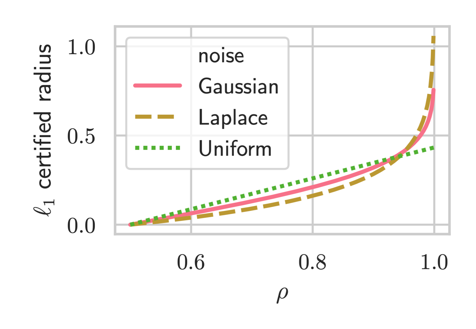
Another way to look at this: Any choice of smoothing distribution $q$ implies a different certified radius against an $\ell_p$ adversary, given a fixed value of $\rho$. For example, below we plot the radii for the $\ell_1$ adversary and for Gaussian, Laplace, and Uniform distributions. What this theorem says is that the slope of the curve at $\rho=0.5$ will be highest for the distribution with Wulff Crystal level sets.

Empirical Results

We ran an extensive suite of experiments on ImageNet and CIFAR-10 to verify our Wulff Crystal theory. In this section we’ll focus on the $\ell_1$ adversary, whose Wulff Crystal is cubical. We therefore compare the following distributions:

1. Uniform (cubical), $\mathbb{I}\{\|x\|_\infty \leq \lambda\}$.
2. Gaussian (non-cubical), $\propto e^{-\|x/\lambda\|_2^2}$.
3. Laplace (non-cubical), $\propto e^{-\|x/\lambda\|_1}$.

We also compare against a larger array of other distributions in our paper, but we shall focus on just the above in this post. We use Wide ResNet for all of our experiments.

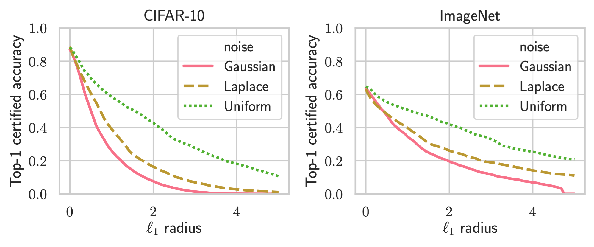
Definition. The certified robust accuracy at an $\ell_p$ radius of $\epsilon$ is the fraction of the test set the smoothed classifier $g$ correctly classifies and certifies robust for at least a ball of size $\epsilon$. Since larger noise variances $\sigma^2 = \mathbb{E}_{\delta\sim q}[\|\delta\|^2_2]$ naturally lead to larger robust radii but trade off against accuracy, we tune over the noise variance and consider the best certified robust accuracy among all values of the hyper-parameter.

Below we show the certified top-1 accuracies for CIFAR-10 and ImageNet. We find that the Uniform distribution performs best, significantly better than Gaussian and Laplace distributions.

Conclusion

In this blog post, we reviewed randomized smoothing as a defense against adversarial examples. We answered the important question of how to choose an appropriate smoothing distribution for a given $\ell_p$ adversary. Empirically, our methods yield state-of-the-art performance for $\ell_1$ robustness. Our paper contains other results that we have not discussed here, like how to calculate robust radii for non-Gaussian distributions and a theorem on the limits of randomized smoothing. We shall cover these in other blog posts, but the reader is welcome to check out the paper in the mean time.

This blog post presented work done by Greg Yang, Tony Duan, J. Edward Hu, Hadi Salman, Ilya Razenshteyn, and Jerry Li. We would like to thank Huan Zhang, Aleksandar Nikolov, Sebastien Bubeck, Aleksander Madry, Jeremy Cohen, Zico Kolter, Nicholas Carlini, Judy Shen, Pengchuan Zhang, and Maksim Andriushchenko for discussions and feedback.