Recently, several works proposed the convolution of a neural network with a Gaussian as a smoothed classifier for provably robust classification. We show that adversarially training this smoothed classifier significantly increases its provable robustness through extensive experiments, achieving state-of-the-art $\ell_2$ provable robustness on CIFAR10 and Imagenet, as shown in the tables below.

Update 09/10/2019: By combining pre-training and semi-supervision with SmoothAdv, we obtain significant improvement over SmoothAdv alone.

$\ell_2$ radius (Imagenet)	0.5	1	1.5	2	2.5	3	3.5
Cohen et al. (%)	49	37	29	19	15	12	9
Ours (%)	56	45	38	28	26	20	17

$\ell_2$ radius (CIFAR-10)	0.25	0.5	0.75	1.0	1.25	1.5	1.75	2.0	2.25
Cohen et al. (%)	61	43	32	22	17	13	10	7	4
Ours (%)	73	58	48	38	33	29	24	18	16
+ Pre-training (%)	80	62	52	38	34	30	25	19	16
+ Semi-supervision (%)	80	63	52	40	34	29	25	19	17
+ Both (%)	81	63	52	37	33	29	25	18	16

We also achieved state-of-the-art $\ell_\infty$ provable robustness on CIFAR10, with $\ell_\infty$ norm $2/255$, as shown in the table below. This is by noting that the $\ell_\infty$ ball of radius $2/255$ is contained in the $\ell_2$-ball of radius $2/255 \sqrt{d} = 2/255 \sqrt{3 \times 32^2} \approx 0.4347$, and invoking our provable robustness for this $\ell_2$ radius.

Model	$\ell_\infty$ Provable Acc @ 2/255	Standard Acc
Ours	68.2	87.2
Carmon et al.	63.8 ± 0.5	80.7 ± 0.3
Wong & Kolter 2018b (single)	53.9	68.3
Wong & Kolter 2018b (ensemble)	63.6	64.1
Interval Bound Propagation	50.0	70.2

Introduction

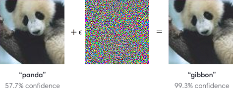
It is now well-known that deep neural networks suffer from the brittleness problem: A small change in an input image imperceptible to humans can cause dramatic change in a neural network’s classification of the image. Such a perturbed input is known as an adversarial example and is by now immortalized in the famous picture below from Goodfellow et al.

As deep neural networks enter consumer and enterprise products of various forms, this brittleness can possibly have devastating consequences (Brown et al. 2018, Athalye et al. 2017, Evtimov & Eykholt et al. 2018, Li et al. 2019). Most strikingly, Tencent Keen Security Lab recently demonstrated that the neural network underlying Tesla Autopilot can be fooled by an adversarially crafted marker on the ground into swerving into the opposite lane.

Adversarial Attack and Defense

Given the importance of the problem, many researchers have formulated security models of adversarial attacks, along with ways to defend against adversaries in such models. In the most popular security model in the academic circle today, the adversary is allowed to perturb an input by a small noise bounded in $\ell_p$-norm, in order to cause the network to misclassify it. Thus, given a loss function $L$, a norm bound $\epsilon$, an input $x$, its label $y$, and a neural network $F$, the adversary tries to find an input $\hat x$, within $\ell_p$-distance $\epsilon$ of $x$, that maximizes the loss $L(F(x), y)$, i.e. it solves the following optimization problem

$\hat x = \argmax_{\|x' - x\|_p \le \epsilon} L(F(x'), y).$

If $F$ has trainable parameters $\theta$, then the defense needs to find the parameters that minimizes $L(F(\hat x), y)$, for $(x, y)$ sampled from the data distribution $D$, i.e. it solves the following minimax problem

$\min_{\theta} \underset{(x, y) \sim D}{\mathbb{E}} L(F(\hat x), y).$

Empirically, during an attack, the adversarial input $\hat x$ can be obtained approximately by solving the max problem using gradient descent, making sure to project back to the $\epsilon$-ball after each step. This is known as the PGD attack (Kurakin et al., Madry et al.), short for “project gradient descent.” During training by the defense, for every sample $(x, y) \sim D$, this estimate of $\hat x$ can be plugged into the min problem for gradient descent of $\theta$. This is known as Adversarial Training, or PGD training specifically when PGD is used for finding $\hat x$.

Empirical Robust Accuracy

Currently, the standard benchmark for measuring the strength of a model’s adversarial defense is the model’s (empirical) robust accuracy on various standard datasets like CIFAR-10 and Imagenet. This accuracy is calculated by attacking the model with a strong empirical attack (like PGD) for every sample of the test set. The percentage of the test set that the model is still able to correctly classify is the empirical robust accuracy.

For example, consider an adversary allowed to perturb an input by $\epsilon = \frac{8}{255}$ in $\ell_\infty$ norm. On an image, this means that the adversary can change the color of each pixel by at most 8 units (out of 255 total) in each color channel — a rather imperceptible perturbation. Currently, the state-of-the-art empirical robust accuracy against such an adversary on CIFAR-10 hovers around 55% (Zhang et al. 2019, Hendrycks et al. 2019), meaning that the best classifier can only withstand a strong attack on about 55% of the samples in CIFAR-10. Contrast this with the state-of-the-art nonrobust accuracy on CIFAR-10 of >95%. Thus it’s clear that adversarial robustness research still has a long way to go.

Provable Robustness via Randomized Smoothing

Note that the empirical robust accuracy is only an upper bound on the true robust accuracy. This is defined by hypothetically replacing the strong empirical attack used in empirical robust accuracy with the ideal attack able to find $\hat x$ exactly for every $x$. Thus, nothing in principle prevents a stronger empirical attack from further lowering the empirical robust accuracy of a model. Indeed, except a few notable cases like PGD (Madry et al.), we have seen most claims of adversarial robustness broken down by systematic and thorough attacks (as examples, see Carlini & Wagner 2016, Carlini & Wagner 2017, Athalye et al. 2017, Uesato et al. 2018, Athalye et al. 2018, Engstrom et al. 2018, Carlini 2019).

This has motivated researchers into developing defenses that can certify the absence of adversarial examples (as prominent examples, see Wong & Kolter 2018, Katz et al. 2017, and see Salman et al. 2019 for a thorough overview of these techniques). Such a defense is afforded a provable (or certified) robust accuracy on each dataset, defined as the percentage of the test set that can be proved to have no adversarial examples in its neighborhood. In contrast with empirical robust accuracy, provable robust accuracy is a lower bound on the true robust accuracy, and therefore cannot be lowered further by more clever attacks. The tables in the beginning of our blog post, for example, display provable robust accuracies on CIFAR-10 and Imagenet.

Until recently, most such certifiable defenses have not been able to scale to large networks and datasets (Salman et al. 2019), but a new technique called randomized smoothing (Lecuyer et al., Li et al., Cohen et al.) was shown to bypass this limitation, obtaining highly-nontrival $\ell_2$ certified robust accuracy on Imagenet (Cohen et al.). We now briefly review randomized smoothing.

Definition

Consider a classifier $f$ from $\mathbb{R}^d$ to classes $\mathcal{Y}$. Randomized smoothing is a method that constructs a new, smoothed classifier $g$ from the base classifier $f$. The smoothed classifier $g$ assigns to a query point $x$ the class which is most likely to be returned by the base classifier $f$ under isotropic Gaussian noise perturbation of $x$, i.e.,

$g(x) = \argmax_{c \in \mathcal{Y}} \; \mathbb{P}(f(x+\delta) = c)$

where $\delta \sim \mathcal{N}(0, \sigma^2 I)$, and the variance $\sigma^2$ is a hyperparameter of the smoothed classifier $g$ (it can be thought to control a robustness/accuracy tradeoff). In Cohen et al., $f$ is a neural network.

Prediction

To estimate $g(x)$, one simply has to

1. Sample a collection of Gausian samples $\delta_i$.
2. Predict the class $y_i$ of each $x + \delta_i$ using the base classifier $f$.
3. Take the majority vote of the $y_i$’s as the final prediction of the smoothed classifier $g$ at $x$.

Certification

The robustness guarantee presented by Cohen et al. is as follows: suppose that when the base classifier $f$ classifies $\mathcal{N}(x, \sigma^2 I)$, the (most popular) class $c_A$ is returned with probability $p_A = \mathbb{P}_\delta(f(x+\delta) = c_A)$, and the runner-up class $c_B$ is returned with probability $p_B = \max_{c \neq c_A} \mathbb{P}_\delta(f(x+\delta) = c)$. We estimate $p_A$ and $p_B$ using Monte Carlo sampling and confidence intervals¹. Then the smoothed classifier $g$ is robust around $x$ within the radius

$\frac{\sigma}{2} \left(\Phi^{-1}(p_A) - \Phi^{-1}(p_B)\right),$

where $\Phi^{-1}$ is the inverse of the standard Gaussian CDF. Thus, the bigger $p_A$ is and the smaller $p_B$ is, the more provably robust $g$ is.

Training

Cohen et al. simply trained the base classifier $f$ under Gaussian noise data augmentation with cross entropy loss, i.e. for each data point $(x, y)$, sample $\delta \sim \mathcal{N}(0, \sigma^2 I)$ and train $f$ on the example $(x+\delta, y)$. With this simple training regime applied to a Resnet-110 base classifier, they were able to obtain significant certified robustness on CIFAR-10 and Imagenet, as shown in our tables.

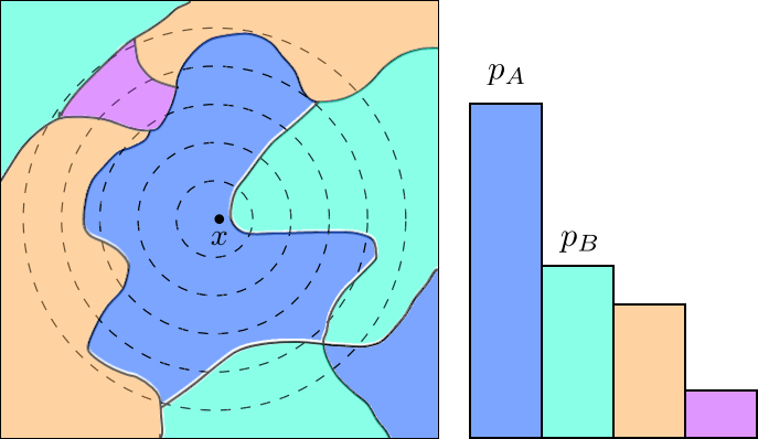
An Illustration

The following figures modified from Cohen et al. illustrate randomized smoothing. The base classifier $f$ partitions the input space into different regions with different classifications, colored differently in the left figure. The regions’ Gaussian measures (under the Gaussian $\mathcal{N}(x, \sigma^2 I)$ whose level curves are shown as dashed lines) are shown as a histogram on the right. The class $c_A$ corresponding to the blue region is the output of the smoothed classifier $g(x)$; the class $c_B$ corresponding to the cyan region is the runner-up class. If $p_A$ is large enough and $p_B$ is small enough, then we can prove that $g(x') = c_A$ for all $\|x' - x\|_2 \le \epsilon$, i.e. $g$ is robust at $x$ for $\ell_2$ radius $\epsilon$.

Adversarially Training the Smoothed Classifier

Intuitively, adversarial training attempts to make a classifier locally flat around input sampled from a data distribution. Thus it would seem that adversarial training should make it easier to certify the lack of adversarial examples, despite having no provable guarantees itself. Yet historically, it has been difficult to execute this idea (Salman et al. 2019, and folklore), with the closest being Xiao et al.

It is hence by no means a foregone conclusion that adversarial training should improve certified accuracy of randomized smoothing. A priori there could also be many ways these two techniques can be combined, and it is not clear which one would work best:

1. Train the base classifier $f$ to be adversarially robust, simultaneous with the Gaussian data augmentation training prescribed in Cohen et al..
2. Find an adversarial example of the base classifier $f$, then add Gaussian noise and train.
3. Add Gaussian noise and find an adversarial example of $f$ in the neighborhood of this Gaussian perturbation. Train $f$ on this adversarial example.
4. Find an adversarial example of the smoothed classifier $g$, then train $g$ on this example.

It turns out that certified accuracies of these methods follow the order (1) < (2) < (3) < (4), with (4) achieving the highest certified accuracies (see our paper). Indeed, in hindsight, if $g$ is the classifer doing the prediction, then we should be adversarially training $g$, and not $f$. In the rest of the blog post, we lay out the details of (4).

Randomized Smoothing for Soft Classifiers

Neural networks typically learn soft classifiers, namely, functions $F: \mathbb{R}^d \to P(\mathcal{Y})$, where $P(\mathcal{Y})$ is the set of probability distributions over $\mathcal{Y}$. During prediction, the soft classifier is argmaxed to return the final hard classification. We therefore consider a generalization of randomized smoothing to soft classifiers. Given a soft classifier $F$, its associated smoothed soft classifier $G: \mathbb{R}^n \to P(\mathcal{Y})$ is defined as

$G (x) = \underset{\delta \sim \mathcal{N}(0, \sigma^2 I)}{\mathbb{E}} F(x + \delta).$

Let $f(x)$ and $F (x)$ denote the hard and soft classifiers learned by the neural network, respectively, and let $g$ and $G$ denote the associated smoothed hard and smoothed soft classifiers. Directly finding adversarial examples for the smoothed hard classifier $g$ is a somewhat ill-behaved problem because of the argmax, so we instead propose to find adversarial examples for the smoothed soft classifier $G$. Empirically we found that doing so will also find good adversarial examples for the smoothed hard classifier.

Finding Adverarial Examples for Smoothed Soft Classifier

Given a labeled data point $(x, y)$, we wish to find a point $\hat x$ which maximizes the loss of $G$ in an $\ell_2$ ball around $x$ for some choice of loss function. As is canonical in the literature, we focus on the cross entropy loss $L_{\mathrm{CE}}$. Thus, given a labeled data point $(x, y)$ our (ideal) adversarial perturbation is given by the formula:

$\begin{aligned} \hat x &= \argmax_{\|x' - x\|_2 \leq \epsilon} L_{\mathrm{CE} } (G (x'), y)\\ &= \argmax_{\|x' - x\|_2 \leq \epsilon} \left( - \log \underset{\delta \sim \mathcal{N} (0, \sigma^2 I)}{\mathbb{E}} F (x' + \delta)_y \right). \end{aligned}$

We will refer to the above as the SmoothAdv objective. The SmoothAdv objective is highly non-convex, so as is common in the literature, we will optimize it via projected gradient descent (PGD), and variants thereof. It is hard to find exact gradients for SmoothAdv, so in practice we must use some estimator based on random Gaussian samples.

Estimating the Gradient of SmoothAdv

If we let $J(x') = L_{\mathrm{CE} } (G (x'), y)$ denote the SmoothAdv objective, then

$\nabla_{x'} J(x') = \nabla_{x'} \left( - \log \underset{\delta \sim \mathcal{N}(0, \sigma^2 I)}{\mathbb{E}} F (x' + \delta)_y \right) \; .$

However, it is not clear how to evaluate the expectation inside the log exactly, as it takes the form of a complicated high dimensional integral. Therefore, we will use Monte Carlo approximations. We sample i.i.d. Gaussians $\delta_1, \ldots, \delta_m \sim \mathcal{N} (0, \sigma^2 I)$, and use the plug-in estimator for the expectation:

$\nabla_{x'} J(x') \approx \nabla_{x'} \left( - \log \left( \frac{1}{m} \sum_{i = 1}^m F (x' + \delta_i)_y \right) \right) \; .$

It is not hard to see that if $F$ is smooth, this estimator will converge to $\nabla_{x'} J(x')$ as we take more samples.

SmoothAdv is not the Naive Objective

We note that SmoothAdv should not be confused with the similar-looking objective

$\begin{aligned} &\phantom{ {}={}} \argmax_{\|x' - x\|_2 \leq \epsilon} \underset{\delta \sim \mathcal{N} (0, \sigma^2 I)}{\mathbb{E}} L_{\mathrm{CE} } (F (x' + \delta), y) \\ &= \argmax_{\|x' - x\|_2 \leq \epsilon} \ \underset{\delta \sim \mathcal{N} (0, \sigma^2 I)}{\mathbb{E}} \left[-\log F(x' + \delta)_y\right] \; , \end{aligned}$

where the $\log$ and $\mathbb{E}$ have been swapped compared to SmoothAdv, as suggested in section G.3 of Cohen et al. This objective, which we shall call naive, is the one that corresponds to finding an adversarial example of $F$ that is robust to Gaussian noise. In contrast, SmoothAdv directly corresponds to finding an adversarial example of $G$. From this point of view, SmoothAdv is the right optimization problem that should be used to find adversarial examples of $G$. This distinction turns out to be crucial in practice: empirically, Cohen et al found attacks based on the naive objective not to be effective. In our paper, we perform SmoothAdv-attack on Cohen et al.’s smoothed model and find, indeed, that it works better than the Naive objective, and it performs better with more Gaussian noise samples used to estimate its gradient.

Adversarially Training Smoothed Classifiers

We now wish to use our new SmoothAdv attack to boost the adversarial robustness of smoothed classifiers. As described in the beginning of this blog post, in (ordinary) adversarial training, given a current set of model parameters $\theta_t$ and a labeled data point $(x_t, y_t)$, one finds an adversarial perturbation $\hat x_t$ of $x_t$ for the current model, and then takes a gradient step for the model parameters $\theta_t$, evaluated at the point $(\hat x_t, y_t)$. Intuitively, this encourages the network to learn to minimize the worst-case loss over a neighborhood around the input.

What is different in our proposed algorithm is that we are finding the adversarial example $\hat x_t$ with respect to the smoothed classifier $G$ using the SmoothAdv objective, and we are training $G$ at this adversarial example $\hat x_t$ with respect to the SmoothAdv objective, estimated by the plug-in estimator.

$\begin{aligned} \theta_{t+1} &= \theta_t + \eta \nabla_\theta \log\left(\frac{1}{m'} \sum_{i=1}^{m'} F(\hat x_t + \delta_i)_y\right), \end{aligned}$

where $\theta_t$ are the parameters of $F$ at time $t$, $\delta_i \sim \mathcal{N}(0, \sigma^2 I)$, and $\eta$ is a learning rate.

More Data: Pretraining and Semisupervision

Hendrycks et al. showed that pre-training on Imagenet can improve empirical adversarial robustness on CIFAR-10 and CIFAR-100. Similarly, Carmon et al. showed that augmenting supervised adversarial training with unsupervised training on a carefully selected unlabeled dataset confers significant robustness improvement. We adopt these ideas for randomized smoothing and confirm that these techniques are highly beneficial for certified robustness as well, especially for smaller radii (though unfortunately their combination did not induce combined improvement). See the tables below.

Results

Over the course of the blog post, we have introduced several hyperparameters, such as 1) $\epsilon$, the radius of perturbation used for adversarial training, 2) $m$, the number of Gaussian noise samples, 3) $\sigma$, the standard deviation of the Gaussian noise. We also did not mention other hyperparameters like $T$, the number of iterations used for PGD iterations, or the usage of DDN, an alternative attack to PGD that has been shown to be effective for $\ell_2$-perturbations (Rony et al.). In our paper we do extensive analysis of the effects of these hyperparameters, to which we refer interested readers.

Taking the max over all such hyperparameter combinations for each $\ell_2$ perturbation radius, we obtain the upper envelopes of the certified accuracies of our method vs the upper envelopes of Cohen et al. in the tables in the beginning of this post, which we also replicate here for convenience.

$\ell_2$ radius (Imagenet)	0.5	1	1.5	2	2.5	3	3.5
Cohen et al. (%)	49	37	29	19	15	12	9
Ours (%)	56	43	37	27	25	20	16

$\ell_2$ radius (CIFAR-10)	0.25	0.5	0.75	1.0	1.25	1.5	1.75	2.0	2.25
Cohen et al. (%)	60	43	32	23	17	14	12	10	8
Ours (%)	74	57	48	38	33	29	24	19	17
+ Pre-training (%)	80	63	52	39	36	30	25	20	17
+ Semi-supervision (%)	80	63	53	39	36	32	25	20	18
+ Both (%)	82	65	52	38	34	30	25	21	18

Conclusion

In this blog post, we reviewed adversarial training and randomized smoothing, a recently proposed provable defense. By adversarially training the smoothed classifier — and carefully getting all the details right — we obtained the state-of-the-art $\ell_2$ provable robustness on CIFAR-10 and Imagenet, demonstrating significant improvement over randomized smoothing alone.

Acknowledgements

This blog post presented work done by Hadi Salman, Greg Yang, Jerry Li, Huan Zhang, Pengchuan Zhang, Ilya Razenshteyn, and Sebastien Bubeck. We would like to thank Zico Kolter, Jeremy Cohen, Elan Rosenfeld, Aleksander Madry, Andrew Ilyas, Dimitris Tsipras, Shibani Santurkar, Jacob Steinhardt for comments and discussions during the making of this paper.