Cross-posted from Microsoft Research Blog

In the pursuit of learning about fundamentals of the natural world, scientists have had success with coming at discoveries from both a bottom-up and top-down approach. Neuroscience is a great example of the former. Spanish anatomist Santiago Ramón y Cajal discovered the neuron in the late 19th century. While scientists’ understanding of these building blocks of the brain has grown tremendously in the past century, much about how the brain works on the whole remains an enigma. In contrast, fluid dynamics makes use of the continuum assumption, which treats the fluid as a continuous object. The assumption ignores fluid’s atomic makeup yet makes accurate calculations simpler in many circumstances.

When it comes to neural networks (NNs), one way to build an understanding is to reason about their behaviors when every layer has infinitely many neurons, commonly known as the NN infinite-width limits. We believe taking a top-down approach, as exemplified in the fluid dynamics example, can lead to a better understanding of why practical wide NNs work and how we can improve them.

The Journey to Infinity

Just like how fluid dynamics under the continuum assumption enables accurate calculations of how real fluid—made of individual atoms—behaves, studying the NN infinite-width limit can inform us about how wide NNs behave in practice. As larger, hence wider, NNs are trained every few months, this will only become truer going forward. The catch, however, is that we need an infinite-width limit that sufficiently captures what makes NNs so successful today. In our paper, “Feature Learning in Infinite-Width Neural Networks,” we carefully consider how model weights become correlated during training, which leads us to a new parametrization, the Maximal Update Parametrization, that allows all layers to learn features in the infinite-width limit for any modern neural network.

There have been two well-studied infinite-width limits for modern NNs: the Neural Network-Gaussian Process (NNGP) and the Neural Tangent Kernel (NTK). While both are illuminating to some extent, they fail to capture what makes NNs powerful, namely the ability to learn features. This is evident both theoretically and empirically. The NNGP limit explicitly considers the network at initialization and trains only a linear classifier on top of untrained features. The NTK limit allows training of the whole network—but only with a small enough learning rate. This means the weights do not leave a small neighborhood of their initialization, preventing the learning of new features. Unsurprisingly, the best-performing NNGP and NTK models underperform their conventional finite-width counterparts, even when we calculate their infinite-width limits exactly.

“Neural Tangent Kernel doesn’t exhibit a critical element of deep learning, which is the ability to learn increasingly abstract features as we add more layers and training proceeds. This work takes an important step toward a theory that captures this capability in overparametrized neural networks.”

— Yoshua Bengio, Professor at the Université de Montréal and Scientific Director at Mila

Figure 1: NNGP and NTK underperform finite-width NNs on Image Classification, Word2Vec and Omniglot, even when calculating their infinite-width limits exactly. This suggests that NNGP and NTK do not capture the learning that happens in a practical NN — that is, they are not the true limit to which finite-width NNs converge. CNN result taken from Arora et al. (2019).

Unlocking Feature Learning by Going Beyond Model Initialization

Why do NNGP and NTK fail to learn features? Because to do so, we need to leave the “comfort zone” of model initialization, where the activation coordinates are easy to analyze as they nicely follow a Gaussian law by a central limit argument—that is, summing infinitely many roughly independent, zero-mean random variables should yield a Gaussian distribution with a known variance. Just like growing a plant entails not only planting a seed but also proper care throughout its lifetime, the right infinite-width limit should take into consideration both the model initialization and the gradient updates, especially far away from initialization. To unlock feature learning, we need to see gradient updates for what they really are: a different kind of matrices from their randomly initialized counterparts.

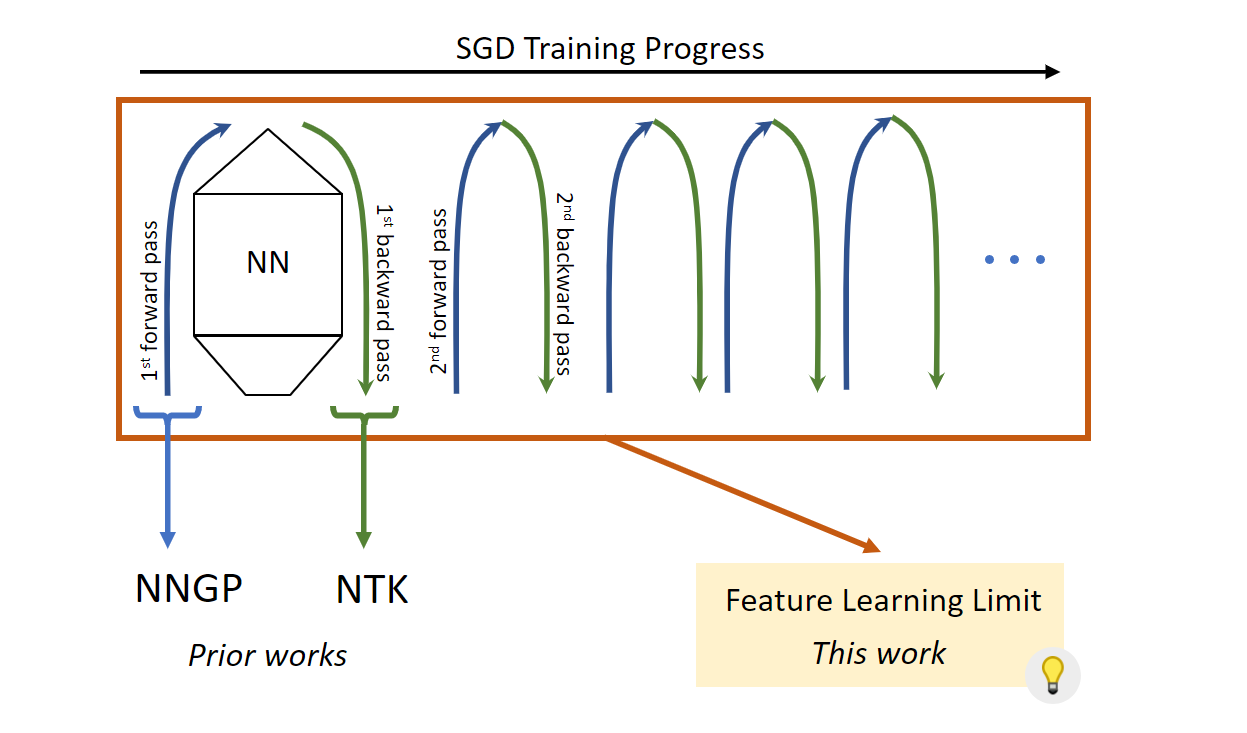
Figure 2: NNGP is essentially the limit of the first forward pass in the training process, and NTK is the first backward pass. Neither leaves the “comfort zone” of model initialization and thus fails to capture feature learning. Our new limit takes into consideration the entire training process, which makes feature learning possible.

When a matrix $W \in \mathbb{R}^{n\times n}$ multiplies with an activation vector $x \in \mathbb{R}^n$ to produce a pre-activation vector, we calculate a coordinate by taking a row from the matrix $W$, multiplying it by $x$ coordinate-wise, and summing the coordinates of the resulting vector. When $W$’s entries are initialized with zero mean, this summation is across roughly independent elements with zero mean. As such, this sum would be $\sqrt{n}$ smaller than what it would be if the elements had nonzero mean or were strongly correlated, due to the famous square root cancellation effect underlying phenomena like the Central Limit Theorem.

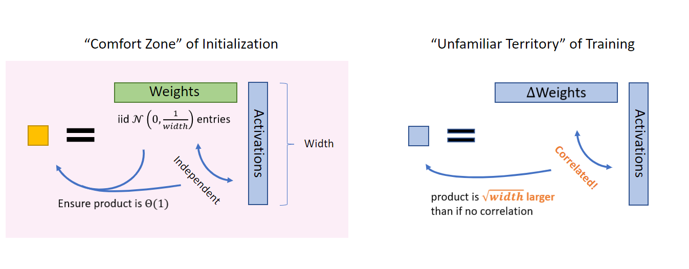
Figure 3: At initialization, the weights are independent from the incoming activations, so their product is easy to reason about (for example, by using Central Limit Theorem); hence, initialization is a “comfort zone.” However, once training starts, the weights (more precisely, the change in weights, ΔWeights, due to the gradient updates) start to correlate with the activations, so we must exit this comfort zone. A Law-of-Large-Number intuition would suggest that their product is $\sqrt{width}$ larger than if there are no correlation.

In fact, this strong correlation occurs after gradient updates to $W$. Let’s focus on the gradient updates themselves, denoted as $\Delta W$. In general, the coordinates of the vector obtained by coordinate-wise multiplying a row from $\Delta W$ and the activation vector $x$ will not have zero mean. This comes partly from the fact that $\Delta W$ “remembers” the data distribution that produces the activations and partly from the model architecture (for example, the use of nonlinearity). Consequently, each entry of $\Delta W x$ will be $\sqrt{n}$ larger than if one naively assumes independence and zero-mean like at initialization.

The key to finding an infinite-width limit that admits feature learning is to carefully analyze when we have sufficient independence and zero mean and when we do not, just like our reasoning above. Now there is just one more step before we can derive such a limit.

Not All Parameters Are the Same

Conventionally, say in a multi-layer perceptron (MLP), we treat all the parameters the same way by using the same initialization, like a Gaussian distribution with a variance of $\frac{1}{fan\_in}$, and the same learning rate. In the infinite-width limit, there are two kinds of parameters with very different behaviors—vector-like parameters and matrix-like parameters.

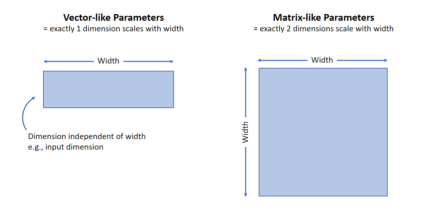
Figure 4: When width is large, two kinds of parameters have different behaviors. Vector-like parameters have exactly 1 dimension scaling with width, while matrix-like parameters have exactly 2 such dimensions.

Vector-like parameters are those with exactly one dimension that scales with width — input or output layer weights and layer biases, for example. Meanwhile, matrix-like parameters have exactly two such dimensions, like hidden layer weights. The key difference is that a matrix multiplication with a vector-like parameter sometimes only sums across the finite, non-width dimension, whereas a matrix multiplication with a matrix-like parameter always sums across the width dimension, which tends to infinity. This distinction is critical in the infinite-width limit — summing infinitely many elements of size $\Theta(1)$ in width produces infinity, while summing finitely many elements each of size $\Theta(1/width)$ produces zero in the limit.

So far, we have introduced two kinds of weights: the random initialization and the gradient updates. We have also introduced two kinds of parameters: the vector-like ones and matrix-like ones. The key is to make sure that all four combinations of these lead the activations to evolve by non-vanishing and non-exploding amounts during training. Maximal Update Parametrization (abbreviated μP) scales the initialization and parameter multipliers as a function of width to ensure it for all activation vectors, thus achieving maximal feature learning. Depending on the model architecture and optimizer used, the actual parametrization could vary in complexity (see abc-parametrization in our paper). However, the underlying principles stay the same.

Practical Impact and Looking Forward

Maximal Update Parametrization (abbreviated μP), which follows the principles we discussed and learns features maximally in the infinite-width limit, has the potential to change the way we train neural networks. For example, we calculated the limit of Word2Vec and found it outperformed both the NTK and NNGP limits as well as finite-width networks. When we visualize the learned embeddings of two groups of words — the names of American cities and those of states — using Principal Component Analysis, we see that μP’s limit exhibits a clear separation between them, like in the finite neural network, while the NTK/NNGP limit sees essentially random embeddings.

“The theory of wide feature learning is extremely exciting and has the potential to change the way the field thinks about large model training.”

— Ilya Sutskever, Co-founder and Chief Scientist at OpenAI

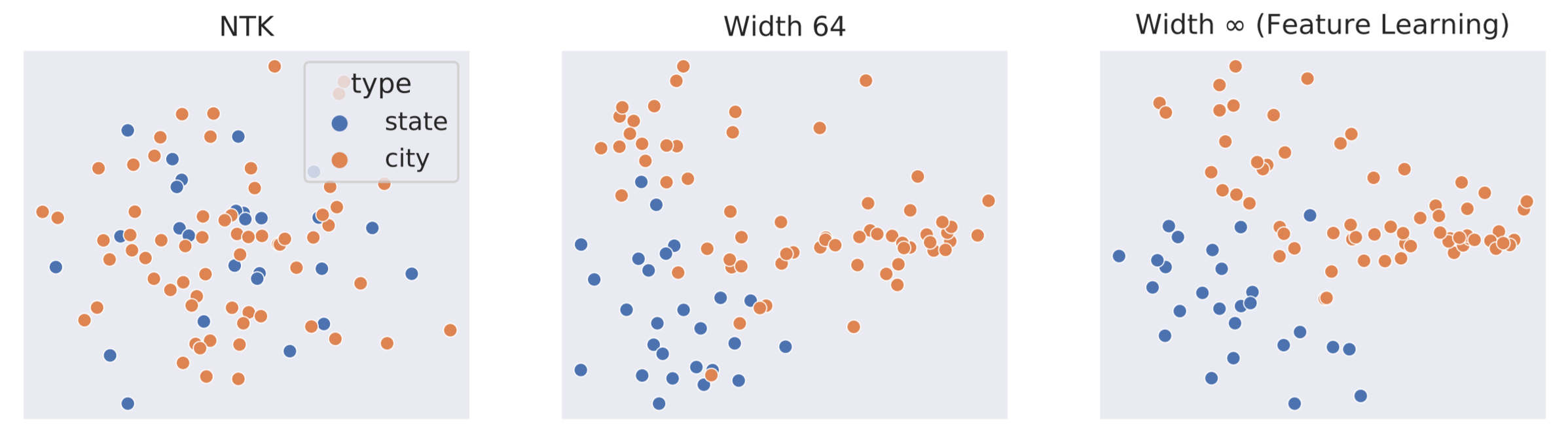
Figure 5: Principal Component Analysis of Word2Vec embeddings of common US cities and states, for NTK, width-64, and width-∞ (feature learning) neural networks. NTK embeddings (left plot) are essentially random — you can see that there is no separation of cities and states in the far left embeddings above. In contrast, cities and states get naturally separated in the embedding space as width increases in the feature learning regime. In the width-64 model (middle plot), some separation can be seen, and even more separation can be seen in the infinite-width model (right plot).

Parametrizing a model in allows it to retain the ability to learn features when its width goes to infinity — that is, the model does not become trivial (like NTK and NNGP) or run into numerical issues in the limit. We believe this new perspective opens doors to new capabilities previously unimaginable. Indeed, our theory enables a novel and useful paradigm for training large models, such as GPT and BERT, which is the topic of one of our on-going projects. Our results also raise several questions about existing practices, for example, about uncertainty in Bayesian neural networks. “These results are also intriguing because they suggest that the infinite width-limit of feature learning leads to a deterministic training trajectory and thus precludes the use of variance due to initialization to ascertain model uncertainty,” Yoshua Bengio explains. “This should inspire future works on better uncertainty estimation in the feature learning regime.”

Due to the dominance of Neural Tangent Kernel theory, many researchers in the community believed that large width causes neural networks to lose the ability to learn features. We decisively refute this belief in our work. However, rather than an end to a chapter, we believe this is just a new beginning with many exciting new possibilities. We welcome everyone to join us on this journey to unveil the mysteries of neural networks and to push deep learning to new heights.

Additional resources:

• Read our paper for a deeper dive into the technical aspects.
• Discover more about feature learning and infinite-width networks in a presentation by Greg Yang.
• Train your own infinite-width feature learning neural network with our GitHub repository.
• Discover questions and comments from the machine learning community on this Reddit thread.